View us on GitHub
Study Overview
Command of language is one of the most significant cognitive abilities we possess and is often the most pervasive signal we encounter in a social media setting. When we notice overt and unintentional grammatical errors in social media posts, do we make unconscious assumptions about the authors’ general intelligence? Do we attribute difficulty with written language with other indicators such as lower-performing verbal acuity or overall intelligence? Further, are some categories of grammatical errors more injurious than others – or do we take in stride all these trespasses?
General intelligence, sometimes referred to as cognitive ability, includes our capacity to ”reason, plan, solve problems, think abstractly, comprehend complex ideas, learn quickly, and learn from experience” (Plomin, 1999). Assessment of our cognitive abilities often informs critical judgments in others that affect our educational, occupational, and relationship opportunities (B. M. Newman & P. R. Newman, 2020). Though social media channels are often used to identify potentially qualified job candidates, their use in screening candidates for suitability and background investigation is also on the rise (Driver, 2020). In the CareerBuilder survey that noted an increase in social media screening, 57% of employers reported rejecting candidates based on negative findings in applicant social media posts. Of those rejected, 27% of employers specified ”poor communication skills” as the primary factor for the rejection.
There is evidence that we ought to take this question seriously. In (Borkenau & Liebler, 1993), college students rated their perceived intelligence of strangers after watching them read aloud a pre-written weather report. The study found a significant correlation between perceived and measured IQ scores of the strangers, suggesting that some information about individual intelligence is provided through verbal communication. (Kreiner et al., 2002) showed that, while experiments with only a small percentage of typographical errors1 didn’t result in significant perceived intelligence ratings, the presence of a larger number of typographical errors or phonological errors did significantly influence the perception of cognitive writing abilities. The participants in these studies were comprised entirely of college students, but it may be the case that other populations would arrive at a different outcome. In (Silverman, 1990) college professors gave equally high perceived intelligence ratings to hypothetical students with and without verbal language difficulties, such as stuttering. More work is necessary to fully understand these questions, particularly in the context of contemporary social media communication channels where abbreviation, punctuation-skipping, and slang are frequently employed to accommodate restrictive post-length limitations on popular platforms.
Based on these previous studies, our experiment seeks to better understand the effect of the two types of spelling errors on perceived intelligence of the writers of social media posts. Our hypothesis is that both typographical and phonological spelling errors, compared to no spelling errors at all, will lead a decreased level of perceived intelligence, irrespective of the nature, content, and platform of the social media post. In addition, we believe that the effect of phonological errors could be greater than typographical errors, both from (Kreiner et al., 2002), and the fact that typographical errors are common in mainstream social media, and do not necessarily reflect the writer's inability to spell the word.
Experiment Design
The purpose of this study is to assess the impact, if any, on the perceived intelligence of authors’ who make spelling errors in social media posts. If the perception of author intelligence is significantly perturbed by such error, it will be useful to know if particular categories of error are more or less deleterious. We will leave outside the scope of this experiment the concern of whether a correlation between spelling error and measured intelligence exists as we are interested only in the potential causal relationship between written error and perception of intelligence.
Our potential outcomes is stated as follows: We compare the average perceived level of intelligence of writers of social media posts when either typographical or phonological spelling errors are made in the post, to what would have happened had the post contained no errors. Since we can only measure one potential outcome (no error, typographical, or phonological), we adopt a pre-test/post-test control group study design (ROXO). In this design, we first randomize participants at the start of the study by allowing each participant an equal chance of being assigned to Control, Typographical, or Phonological. Next, all participants are measured on one post (identical for all groups, and containing no errors -- more details of measurement below) in order to establish a pretreatment baseline across all individuals. Each group is then subjected to their particular treatment for 5 more posts (Control receives posts with no error, Typographical receives posts with only what's deemed typographical error, and Phonological receives only what's deemed phonological error). We then measure the participants responses after each post. Our null and alternative hypotheses are stated as follows:
H0: In a comparison of individuals, those who are exposed to either treatment (typographical or phonological errors) will not view its author as less intelligent than those exposed to control (no errors).
H1: In a comparison of individuals, those who are exposed to either treatment (typographical or phonological errors) will view its author as less intelligent than those exposed to control (no errors).
In order to establish that our randomization processed worked correctly, we perform a covariate balance check using the R package "cobalt". We check all covariantes not related to the pretreatment (this will be done later with a placebo test), including demographic information, and how often individuals in each group reads and writes social media posts. This check measures raw differences in proportion for categorical variables across the control and treatment groups. For example, for how often an individual reads social media, we have 5 potential levels ("Weekly", "Less than Weekly", "Daily", "More than once a day", and "Prefer not to say"). The difference in proportion of individuals belonging to these levels is calculated across all three groups. There's indication that this raw difference is a strong predictor of potential bias, and that a threshold of 0.1 to 0.25 have been proposed to be satisfactory. Our check (see our analysis notebook for more details) indicates that 36 / 39 levels of our covariates pass the balance check at a threshold level of 0.1, while the remaining 3 pass the level of 0.15. Two of these three are levels of how often one reads social media ("Daily" at 0.1575, "More than once a day" at 0.1022), and one is how often one writes social media ("Less than Weekly" at 0.1476). All other levels of these variables pass the 0.1 threshold. Due to such small differences in only a few levels of two variables, and the fact that all are below or signficantly below the acceptable threshold of 0.25, we believe the covariate balance check passes in our case since. Bias in our estimates should not be an issues in terms of including these covariates in our analysis.
Participants
Our study recruited volunteer survey participants through a combination of social media posts on Facebook and Slack for conducting a Pilot study. Following the pilot, the formal experiment will recruit through a combination of Amazon Mechanical Turk (Mar 31, 2021 - Apr 1, 2021) and the University of California, Berkeley XLab (Apr 5, 2021 - Apr 9, 2021). Data collected after this date (about 40 additional response) were intentially not reported, as we had already started our analysis and did not want our knowledge of the majority of the dataset to influence decisions we make on this remaining data. However, as a disclaimer, including this additional data did not change any of our reported conclusions. The survey ran as omnibus alongside other experiments on a variety of topics being researched during the Spring 2021 semester at the UC Berkeley MIDS program; all demographic data was shared as common resource for each sub-survey.
Pilot Study
Our pilot was conducted on Mar 10, 2021 - Mar 11, 2021; open solicitations were posted on public walls and message boards accessible to the study organizers, including Facebook and UC Berkeley's Slack. Randomization into one of three branches {Control, Treatment A (typographical errors), Treatment B (phonological errors)} occurred at the point of accessing the static web app that redirects to the desired survey forms. Survey's were written in Microsoft Office Forms product and data for each branch was collected on March 11, 2021 at the close of the pilot.
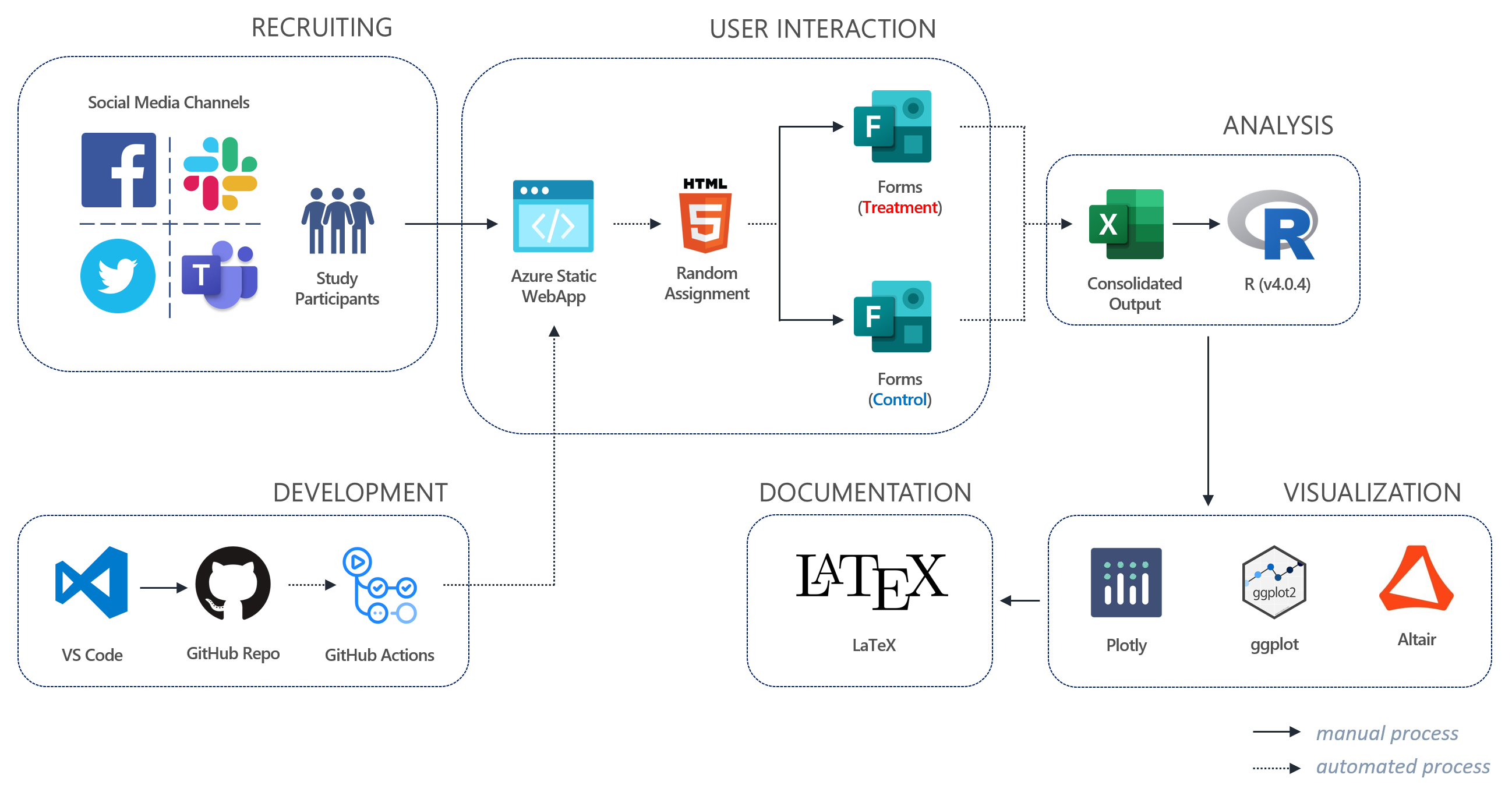
Our Pilot Study Architecture
Pilot randomization
To establish randomization as close to the point of survey as possible, all participants were redirected at the moment just prior to survey initiation via a static web app call using javascript as follows:
  <!-- Randomization Code for Study Participants -->
  <script>
    var urls = ["<control group url>", "<treatment group A url>", "<treatment group B url>"];
    window.location.href = urls[Math.floor(Math.random() * urls.length)];
  </script>
Pilot Participation
We received participation from 31 volunteers for our pilot study between Mar 10, 2021 - Mar 11, 2021. Through randomization, assignment to control and treatment groups were as follows:
Despite having only a small pilot dataset to work with, we had a very noteable result in our regression analysis. We employed a simple linear model of treatment against the intelligence outcome of interest, and controlled for each question to allow for separate means. The results showed high statistical sigificance between our treatment groups and control, with phonological having more than double the effect of typographical.
NOTE: We removed Q4 (i.e., '
Nature') from the live study because the length of post was universally regarded as too long by the experiment organizers and pilot study participants. Accuracy of measuring an effect requires that we encourage participants to read the entire post, and Q4 was discouraging that behavior. Therefore, results here do not include Q4, BUT if we did include Q4, the results remains the same (highly statistically significant) with even slightly more negative coefficient estimates.
| Dependent variable: | |
| Intelligence | |
| TypeP | -1.567*** |
| (0.283) | |
| TypeT | -0.726*** |
| (0.226) | |
| factor(q_num)2 | -0.677** |
| (0.321) | |
| factor(q_num)3 | -1.065*** |
| (0.321) | |
| factor(q_num)5 | -0.516 |
| (0.321) | |
| factor(q_num)6 | -0.387 |
| (0.321) | |
| Constant | 4.962*** |
| (0.261) | |
| Observations | 155 |
| R2 | 0.227 |
| Adjusted R2 | 0.196 |
| Residual Std. Error | 1.265 (df = 148) |
| F Statistic | 7.243*** (df = 6; 148) |
| Note: | *p<0.1; **p<0.05; ***p<0.01 |
Live Study
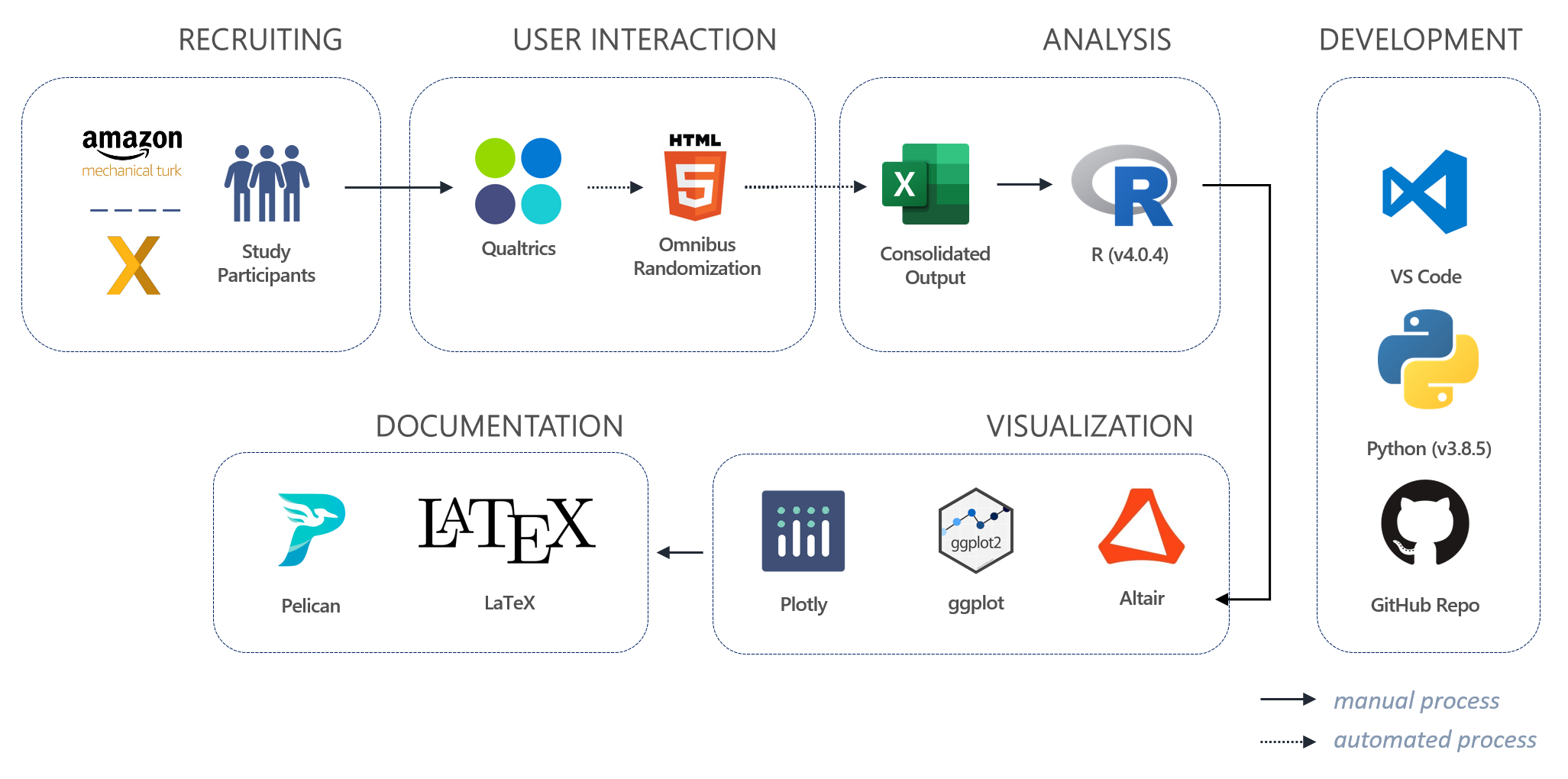
Our live study was conducted between Mar 31, 2021 - Apr 9, 2021, divided into two main sections: Amazon Mechanical Turk participants had access from Mar 31, 2021 through Apr 1, 2021 and UC Berkeley XLab participants had access to the omnibus survey from Apr 6, 2021 through Apr 9, 2021. Randomization and survey execution was carried through Qualtrics as depicted below.
Our Live Study Architecture
Live Study Participation
In our live study, we collected survey feedback from a total 265 participants, with the vast majority coming from Qualtrics (209 or ~78.9%); the remaining came from participants recruiter through Amazon Mechanical Turk (56 or ~21.1%). The balance of group assignment came out to be nearly uniform, with a slight advantage to control group.
Methodology
Participants were invited to join a short, anonymous survey with the communicated intent of assessing their opinion on the appropriateness in length of social media posts. Deception was employed to avoid anticipated response bias in individuals who may occasionally commit typographical or phonological errors themselves and thus may, when asked to consciously consider the intelligence of those who commit errors, provide a more charitable rating. After collection of basic and shared demographic data, participants are presented with a series of seven example social media posts individual followed by eight questions [for each example post]. The questions are delivered in the following order and category:
- Attention Question
- Recall question about the content of the social media post
- Decoy Questions
- 5-point Likert question about the appropriateness in length of the social media post
- 7-point Likert question about attitude toward content of post
- Outcome of Interest Questions
- 7-point Likert question asking if author was 'effective' in communicating their message
- 7-point Likert question asking the participants opinion on the 'intelligence' of the author
- 7-point Likert question asking the participants opinion of the author's 'writing skills'
- Decoy Question
- 7-point Likert question asking what the level of interest is in meeting the author
- Attention Question
- Question asking for how many spelling or grammar mistakes the participant noticed
Treatment Experience
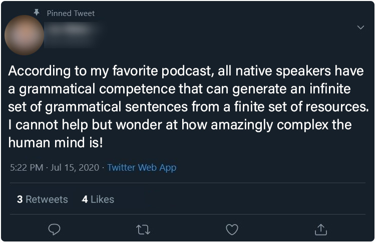
For our study, we constructed seven fictive social media posts: one a control question that everyone receives, regardless of branch assignment, and six posts that are identical in content save for deliberate typographical errors (treatment group 1), or deliberate phonological errors (treatment group 2). The control question contains no grammatical or spelling errors, and is presented as the first question for all participants as a mechanism to prime the participants for attention and to elicit more careful reading of the following five posts. While control group postings are meant to avoid grammar and spelling mistakes, some loose language is used to establish credibility as 'genuine' to a normal social media interaction. All posts cover topics that are intended to be banal so as to avoid evocation of excited emotional states [we assume there to be] due to topics such as religion or politics.
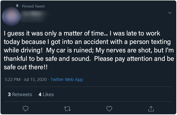
Attention Social Media Post (Post 0) - All Participants
The control post (dubbed Post 0) in our experiment that all assignment groups see first to prime participant focus and attention.

Control Group : Posts 1 - 6
Below, the six posts seen only by the control group participants. Click on any image to see a full-sized version
| Post 1 | Post 2 | Post 3 |
 |
 |
 |
| Post 4 | Post 5 | Post 6 |
 |
 |
 |
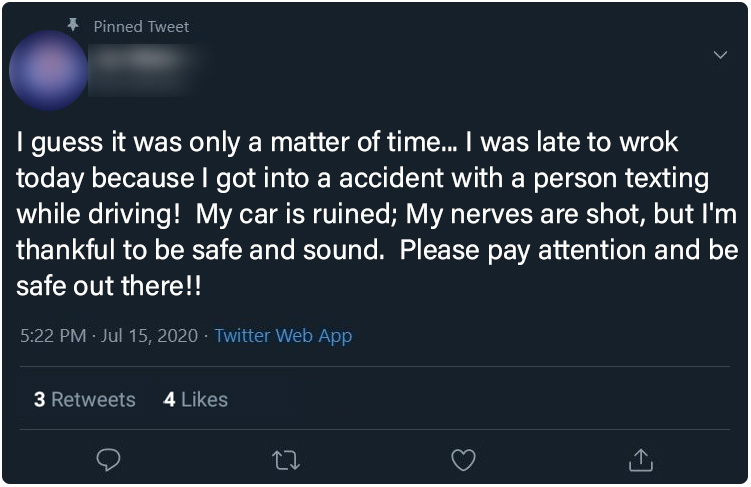
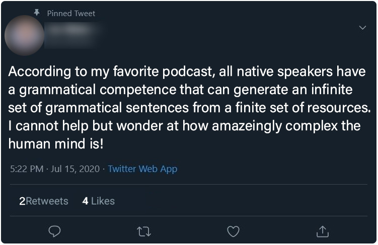
Treatment Group 1 (Typographical) : Posts 1 - 6
Below, the six posts seen only by treatment group 1 (typographical errors) participants. Click on any image to see a full-sized version
| Post 1 | Post 2 | Post 3 |
 |
 |
 |
| Post 4 | Post 5 | Post 6 |
 |
 |
 |
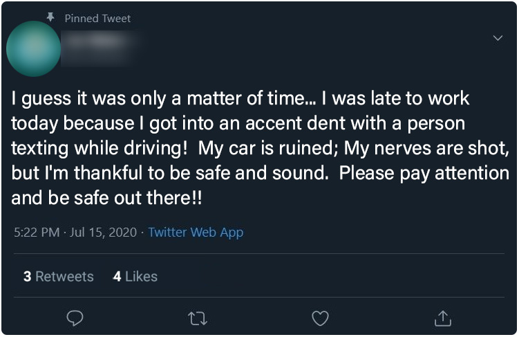
Treatment Group 2 (Phonological) : Posts 1 - 6
Below, the six posts seen only by treatment group 2 (phonological errors) participants. Click on any image to see a full-sized version
| Post 1 | Post 2 | Post 3 |
 |
 |
 |
| Post 4 | Post 5 | Post 6 |
 |
 |
 |
Pre-Survey Power Analysis
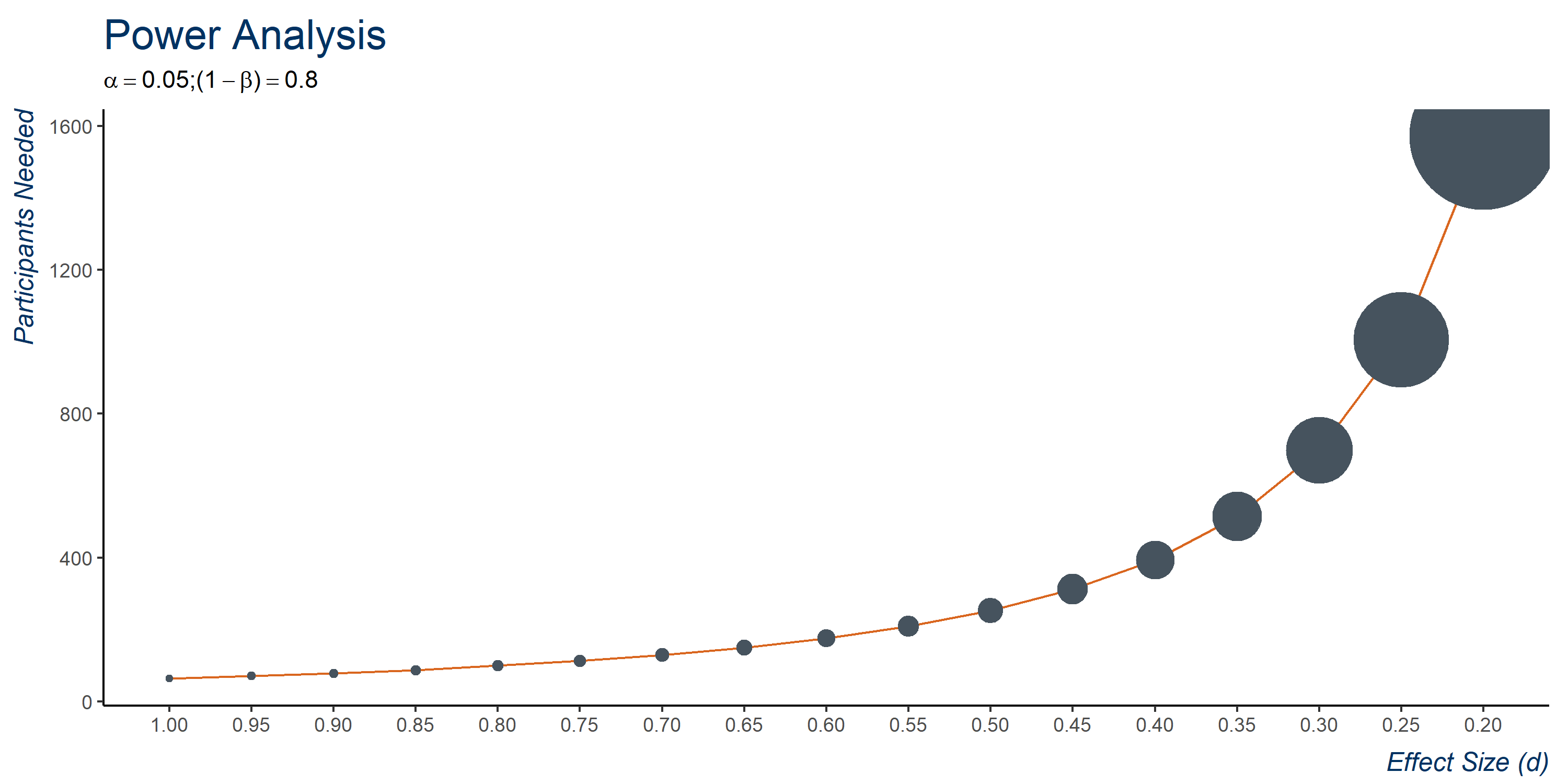
Prior to conducting the experiment, we performed a power analysis to estimate the number of compliant study participants we would need to reach our desired Beta = 0.8 and alpha = 0.05. Below is the code in R we used to perform our pre-experiment power analysis. For a range of effect sizes, going from 0.2 to 1 (where effect size is the average difference in mean perceived Intelligence between either treatment or control), we calculate the number of participants needed using the R package "pacman" using a standard t-test in order to achieve our desired error rates.
if (!require("pacman")) install.packages("pacman")
pacman::p_load(pwr, ggplot2, install = TRUE)

effect_sizes <- seq(0.2,1.0,0.05)
participants_needed <- vector(mode="logical", length=length(effect_sizes))

l <- 1
for (j in effect_sizes){
  participants_needed[l] <- ceiling(pwr.t.test(d = j/2, power = 0.80, sig.level = 0.05)$n)
  l <- l + 1}

results <- data.table(
  effect_size = effect_sizes,
  participants_needed = participants_needed)
A visual of the results is presented below. We see that for very small effect sizes of <0.25, over 1000 subjects would be needed. For a still conservative effect size of 0.5 (keeping in mind our Intelligence scale ranges from 1-7), we would approximately need between 250-300 participants to meet our desired power and significance goals, which is something XLab is able to provide.
Flow diagram
Below is our CONSORT document showing the flow of our study. With 265 recruited individuals, 209 were included in the final analysis from UCB XLab.
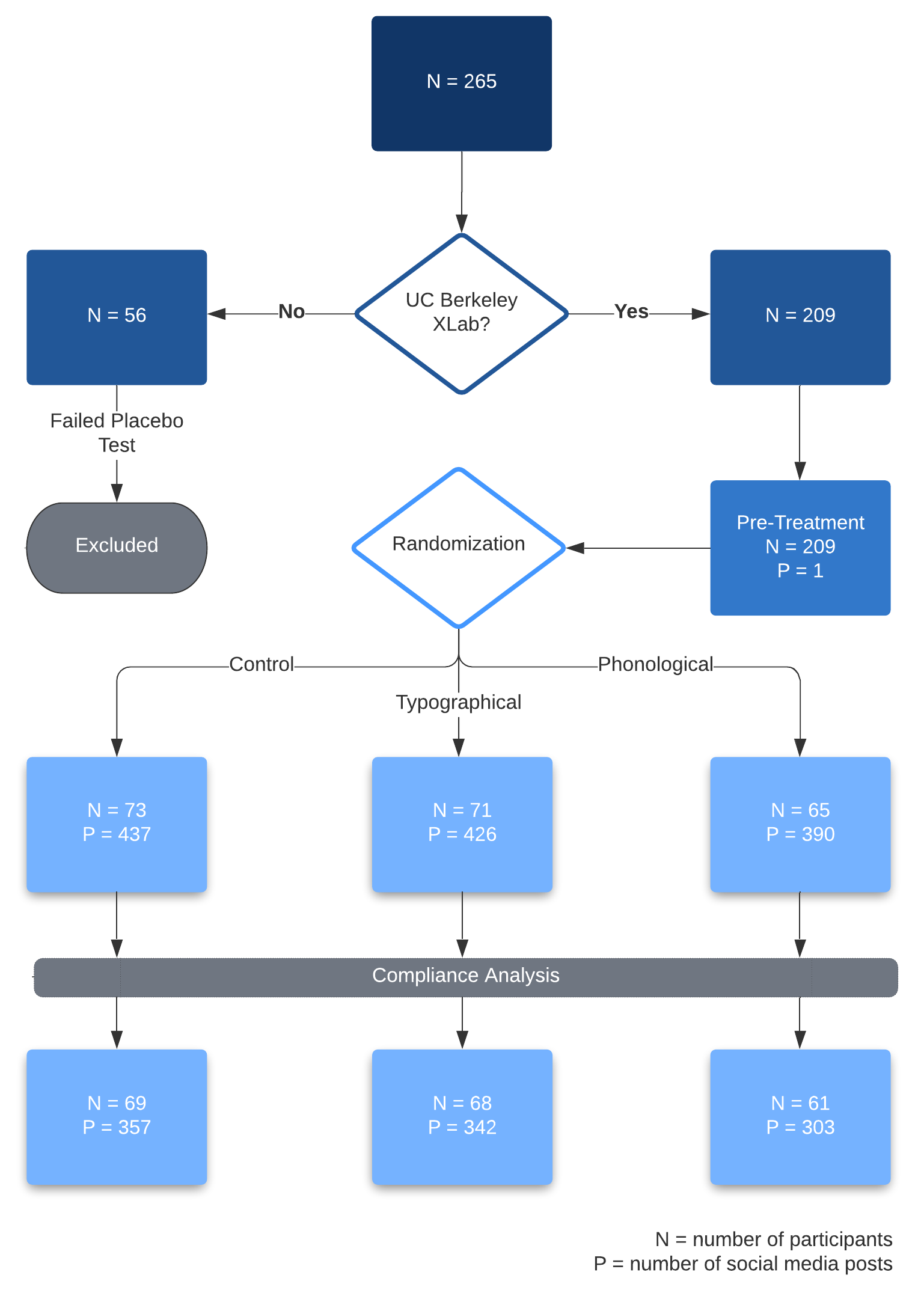
In the first part of the analysis, we consider compliance as a non-issue as all participants had the opportunity to read their respective posts and thus receive either control or treatment. However, even though treatment was always delivered, whether it made actually made an impression on the reader is a different question. In order to gauge this, our final "Attention Question" gauged whether participants noticed spelling errors when they were supposed to (both treatment groups), and did not notice spelling errors when they were not supposed to (control group). While this measurement is a noisy metric for true compliance, if it were a perfect metric, we potentially have two-sided noncompliance (some Control subjects noticed errors, and some Treatment subjects did not notice errors). The CONSORT document shows our fraction of compliers, and number of prompts that falls within our compliance parameters. We deal this further with an instrumental variables approach in the analysis.
Exploratory Data Analysis
Below is a summary analysis of relevant findings in the preliminary exploration of the live study data. Pilot data has not been included here for brevity. NOTE: This section is not an exhaustive EDA; rather, it is focused on showing errata and interesting findings only.
Demographics
Demographic data was collected at the beginning of the ominbus study for all experimentation teams; as such, the questions asked are a composite of the questions formulated by the individual teams during research design. Unfortunately, some data elements were captured via free-form text entry rather than a radio-button, drop-down, or other fixed selection mechanism and resultantly some of the data has mistaken entries or missing values. Below is a distribution of the demographic data present in the omnibus results files:
Distribution of Missing Demographic Data
| % Missing Values | Missing Values | Non-Null Values | Density | |
|---|---|---|---|---|
| Year | 0.69 | 11 | 1576 | 0.03 |
| Gender | 0.00 | 0 | 1587 | 0.17 |
| English | 0.00 | 0 | 1587 | 0.33 |
| Race | 0.00 | 0 | 1587 | 0.12 |
| Country | 1.83 | 29 | 1558 | 0.08 |
| State | 9.77 | 155 | 1432 | 0.04 |
| Student | 0.38 | 6 | 1581 | 0.20 |
| Degree | 0.00 | 0 | 1587 | 0.25 |
Demographic: YEAR
The YEAR variable was intended to capture the calendar year of the study participants birth; of the 265 study participants in the live study, only 255 had valid entries; their distribution is depicted below.
Ten of the entires in YEAR, which was presented to the participant as a free-form text box, are invalid as-is:
# df contains a pandas dataframe with the live study survey data
df2 = df.copy()
df2.Year = df2.Year.fillna('<MISSING>')
df2 = pd.DataFrame(df2.groupby(by=['ROWID','Year']).size()\
    .reset_index()[['ROWID','Year']].Year.value_counts(dropna=False))\
    .reset_index().rename(columns={'index':'year', 'Year':'count'}).sort_values(by='year')

strange_values = ['19996','25','26','54','<MISSING>','Los Angeles','Mumbai, India','US','2020']
df2[(df2.year.isin(strange_values))].year.unique()
Results:
array(['19996', '2020', '25', '26', '54', '<MISSING>', 'Los Angeles', 'Mumbai, India', 'US'], dtype=object)
Demographic: GENDER
GENDER data was provided by the study participant through selection of a single-select radio button choice menu. In our data, Cisgender Women drastically outweigh the rest of the combined genders; this may be the result of Cisgender Woman being the first option in the menu (and thus was selected by 'default' whereby the participant did not change the option). The option Transgender Woman was presented to the study participants, but was not selected.
Demographic: COUNTRY
The COUNTRY variable represents the birth country of the study participant. The vast majority of participants in our study were from the United States of America; however, we did have five missing values in the field, indicating the study participant either did not want to provide one or elected not enter it for another reason.
Demographic: STATE
A total of 25 unique U.S. States were represented in the demographic data identifying the birth state of those participants born in the United States. The vast majority of those who participated in the survey were from California; 26 participants did not specify a state during the demographic section of the survey. Fortunately, all 26 missing states are for participants with a missing or non-US country listed as their birth country.
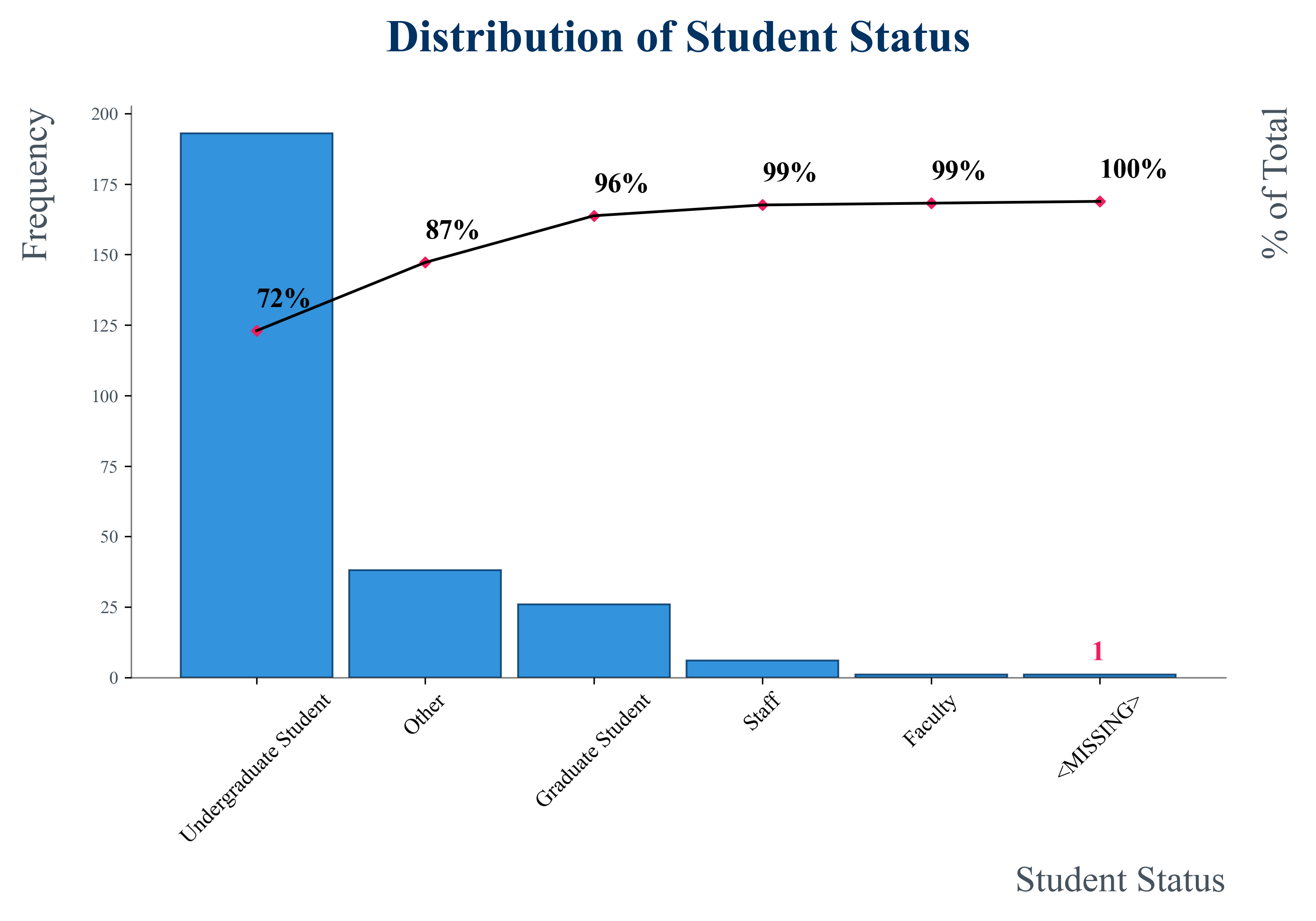
Demographic: STUDENT
The majority of respondants (approximately ~72%) were undergraduate students, with a small mix of Other, Graduate Student, Staff, and Faculty represented. Only one missing value for student status was found in the demographic portion of the survey data.
Survey Response Data
Findings from response data from the live survey is outlined in this section. Analysis will generally be performed by displaying response data for that collected through Amazon Mechanical Turk and data collected from UC Berkeley XLab separately.
Descriptive Statistics
Below are descriptive statistics for the response data of interest. We present two tables showing the descriptive statistics associated with our Mechanical Turk and XLab datasets. Numbers in dark blue shading mark the highest values in each column while lighter blue shading marks the next highest values. The takeaway here is that most users processed our survey at times that we expected the survey, judging from the median values for our words per minute calculator and the time spent on our prompts; roughly 13 minutes for our social media posts and 24 minutes for our questions. On the XLab data, responses for all post-treatment (Interest through Meet) questions ranged the entire scale from 1-7, indicating desirable high variability in the responses at least in the extremes. For the measurement of interest (Intelligence), the avereage is right around the middle of the scale at 3.96.
Descriptive Statistics : Amazon Mechanical Turk
| count | mean | std | min | 25% | 50% | 75% | max | |
|---|---|---|---|---|---|---|---|---|
| PromptTime | 334.00 | 30.16 | 75.98 | 0.74 | 9.38 | 15.29 | 25.93 | 967.12 |
| QuestionTime | 334.00 | 43.90 | 74.77 | 5.86 | 19.31 | 28.61 | 46.65 | 1114.19 |
| wpm | 334.00 | 395.53 | 574.86 | 3.23 | 122.29 | 209.68 | 346.46 | 3913.04 |
| Interest | 334.00 | 3.97 | 1.64 | 1.00 | 3.00 | 4.00 | 5.00 | 7.00 |
| Effective | 334.00 | 4.60 | 1.41 | 1.00 | 4.00 | 5.00 | 6.00 | 7.00 |
| Intelligence | 334.00 | 4.55 | 1.40 | 1.00 | 4.00 | 5.00 | 6.00 | 7.00 |
| Writing | 334.00 | 4.33 | 1.50 | 1.00 | 3.25 | 4.00 | 5.00 | 7.00 |
| Meet | 334.00 | 3.68 | 1.79 | 1.00 | 2.00 | 4.00 | 5.00 | 7.00 |
Descriptive Statistics : Berkeley XLab
| count | mean | std | min | 25% | 50% | 75% | max | |
|---|---|---|---|---|---|---|---|---|
| PromptTime | 1253.00 | 18.17 | 47.53 | 0.54 | 9.22 | 13.29 | 19.28 | 1570.79 |
| QuestionTime | 1253.00 | 30.20 | 51.57 | 7.81 | 18.05 | 23.56 | 31.38 | 1432.50 |
| wpm | 1253.00 | 347.49 | 428.14 | 1.83 | 165.30 | 241.83 | 356.52 | 5423.73 |
| Interest | 1253.00 | 2.90 | 1.68 | 1.00 | 1.00 | 3.00 | 4.00 | 7.00 |
| Effective | 1253.00 | 4.65 | 1.65 | 1.00 | 4.00 | 5.00 | 6.00 | 7.00 |
| Intelligence | 1253.00 | 3.96 | 1.47 | 1.00 | 3.00 | 4.00 | 5.00 | 7.00 |
| Writing | 1253.00 | 3.62 | 1.50 | 1.00 | 3.00 | 4.00 | 5.00 | 7.00 |
| Meet | 1253.00 | 2.64 | 1.57 | 1.00 | 1.00 | 2.00 | 4.00 | 7.00 |
Questionable Responses
There were a number of dubious responses in the data that indicated less than serious attention; from uniform likert-scale choices to implausible response times. In this section, we'll highlight a few of the data issues that gave us pause as to how to proceed.
Variance in Likert Scale Responses
When survey takers are presented with a cluster of vertically-stacked likert scale questions, a common shortcut tactic is to simply vertically click down a column of the questions without considering their intent. In our study, we present a five-question cluster of this sort for each of the six social media posts presented. If a survey participant is fatiqued or disinterested, they may select "all 1's" or "all 7's" as a way to complete their task as soon as possible. Only three of our five questions are "similar" in their scope and thus the liklihood that a careful participant would, after due consideration, select a uniform distribution of these values is relatively low.
Thus, we can use signal from zero variance responders, along with other information about response times and reading words-per-minute, to handle potentially noisy and meaningless responses.
Further, we noticed variance in the rate of uniform response; some participants only exhibit this behavior once while others uniformly select a value every time they are presented with a survey question:
We also noticed a troubling trend in response time of some participants in the form of expressed words per minute as calculated below, where length is the length in each social media post in words, and PromptTime is the time in seconds spent by the participant on the single page presenting the post image (presumably, the participant is reading the post during this time).
study_data[, wpm := length/(PromptTime/60)]
According to a speed-reading test sponsored by Staples as part of an e-book promotion, the average adult reads at a rate of 300 wpm. Per the same study, college professors read at an average of 675 wpm and the world speed reading champing attained 4700 wpm in a controlled competition. Somehow, we managed to elicit responses from participants performing far above these metrics... or, more likely, we have participants who are skimming or simply skipping the reading altogether:
Data Cleaning and Covariates
Details of our data cleaning process is outlined in our analysis notebook, but we describe the specifics related to our outcome variable and covariates here. Our outcome (Intelligence) is coded from a 1-7 Likert scale variable. For the experimental analysis presented here, we treat this variable as numerical, but show later on with Bayesian analysis that the type of model (in particular an ordinal response model) does not influence our conclusions. Most of our covariates as used is from the experiment, but a few have been redesigned. Namely, for geographic location, the vast are in the U.S., with a few scattered across the world. We use an indicator isUS to indicate whether the participant is in the U.S. For age bins, we binned based on 18-25, 26-30, 31-35, 36-40, and 40+.
Placebo Tests
In order to assess the quality of the source data provided by both Amazon Mechanical Turk and UC Berkeley XLab, we performed placebo tests by measuring the impact of treatment on our pretreatment control question (i.e., Post 0 referenced above). The results indicate that there is a very statistically significant treatment effect for the Mechincal Turk data, giving rise to the suspicion that the quality of this data may warrant abandoning it completely. To generate the placebo tests and comparisons, we performed the following steps:
# Placebo tests : Intelligence (of pretreatment question) ~ Treatment for both Amazon and XLab
model_mechturk_control <- control_q[isMechTurk == 1, lm(Intelligence ~ Treatment)]
model_ucb_control <- control_q[isMechTurk == 0, lm(Intelligence ~ Treatment)]
# Generate robust standard errors
robust_MT <- sqrt(diag(vcovHC(model_mechturk_control, type = "HC1")))
robust_UCB <- sqrt(diag(vcovHC(model_ucb_control, type = "HC1")))
# produce placebo model comparison between Amazon and XLab
stargazer(model_mechturk_control, model_ucb_control,
          se = list(robust_MT, robust_UCB), type="html", column.labels = c("Amazon", "XLab"))
A comparison of the models are below:
| Dependent variable: | ||
| Intelligence | ||
| Amazon | XLab | |
| (1) | (2) | |
| TreatmentPhonological | 0.911** | -0.032 |
| (0.393) | (0.204) | |
| TreatmentTypographical | 0.244 | -0.190 |
| (0.450) | (0.226) | |
| Constant | 4.200*** | 3.740*** |
| (0.278) | (0.159) | |
| Observations | 56 | 209 |
| R2 | 0.083 | 0.004 |
| Adjusted R2 | 0.049 | -0.005 |
| Residual Std. Error | 1.313 (df = 53) | 1.268 (df = 206) |
| F Statistic | 2.404 (df = 2; 53) | 0.459 (df = 2; 206) |
| Note: | *p<0.1; **p<0.05; ***p<0.01 | |
Intelligence Measurements (XLab Only)
In the divergence plots below, we look at the aggregate votes along the three outcome of interest questions from our survey sectioned by which group participants were assigned. As the data from Amazon Mechanical Turk was evaluated to be of dubious quality, only results from the XLab experiments is included.
Did the author effectively communicate their message?
Do you think the author has strong writing skills?
What is your judgment of the author's intelligence?
Regression Analysis
Baseline model
We begin with a baseline model looking at only the effect of treatment against perceived level of intelligence. Throughout this report, we will use robust standard errors in order to generate our p-values. Our treatment variable has 3 levels, control, typographical treatment, and phonological treatment. Both treatment levels are negative compared to "control", indicating that individuals perceive the authors to be less intelligent when typos are present in the writing. The estimate for "phonological" is more negative than "typographical" at more than double the magnitude, indicating that misspellings based on the sound of a word ("Kansus" vs "Kansas") has a stronger effect than accidentical typos ("how" vs "hwo"). Both are highly statistically significant with near 0 p-values, indicating that with 95% confidence, we believe the true mean is not 0. For phonological, we estimate a 1.142 decrease in average perceived intelligence on our 7 point scale compared to control, whereas for typographical, we observed a 0.558 decrease.
| Dependent variable: | |
| Intelligence | |
| Baseline | |
| TreatmentPhonological | -1.142*** |
| (0.108) | |
| TreatmentTypographical | -0.558*** |
| (0.104) | |
| Constant | 4.563*** |
| (0.067) | |
| Observations | 1,044 |
| R2 | 0.095 |
| Adjusted R2 | 0.093 |
| Residual Std. Error | 1.433 (df = 1041) |
| F Statistic | 54.481*** (df = 2; 1041) |
| Note: | *p<0.1; **p<0.05; ***p<0.01 |
Model with demographic covariates
Next, we control for demographic variables as well as properties of the post. Each post was shown in the same order to all participants, so there's no variation on that front. We used the length of the post as a covariate. We had 8 demographic variables, including gender (using cisgender female as the base level), whether English is the participant's primary language, race, and highest level of degree obtained. We also have an indicator for whether the individual is located in the United States, along with 5 age bins. We also included the author's self-reported level of social media interaction, including how often individuals read and write social media posts. These were collected pretreatment. By including these covariates, we see that the estimates for treatment effect for both typographical and phonological increases, while the standard errors stay about the same. "Length" of the post is a statistically significant variable that is negative, indicating that the longer the post, the overall lower level of perceived intelligence. Other variables have some significant levels, but are mostly non-significant.
| Dependent variable: | ||
| Intelligence | ||
| Baseline | Demographics | |
| (1) | (2) | |
| TreatmentPhonological | -1.142*** | -1.260*** |
| (0.108) | (0.108) | |
| TreatmentTypographical | -0.558*** | -0.637*** |
| (0.104) | (0.109) | |
| length | -0.028*** | |
| (0.003) | ||
| GenderCisgender Man | -0.160 | |
| (0.103) | ||
| GenderNon-binary | -0.262 | |
| (0.184) | ||
| GenderOther | 1.833*** | |
| (0.270) | ||
| GenderPrefer not to disclose | -1.274*** | |
| (0.471) | ||
| GenderTransgender Man | 0.921*** | |
| (0.295) | ||
| EnglishPrefer not to say | 0.424 | |
| (0.331) | ||
| EnglishYes | -0.030 | |
| (0.110) | ||
| RaceBlack or African American | 0.311 | |
| (0.281) | ||
| RaceHispanic or Latino | 0.118 | |
| (0.157) | ||
| RaceNative Hawaiian or Pacific Islander | 0.083 | |
| (0.714) | ||
| RaceNon-Hispanic White | -0.065 | |
| (0.122) | ||
| RaceOther: | -0.277 | |
| (0.187) | ||
| RacePrefer not to answer | 0.076 | |
| (0.294) | ||
| isUS | -0.161 | |
| (0.183) | ||
| DegreeBachelor's degree | -0.121 | |
| (0.383) | ||
| DegreeNo college | -0.328 | |
| (0.379) | ||
| DegreeSome college | -0.176 | |
| (0.374) | ||
| age_bins18-25 | 0.095 | |
| (0.635) | ||
| age_bins26-30 | -0.009 | |
| (0.681) | ||
| age_bins31-35 | 0.042 | |
| (0.993) | ||
| age_bins41+ | -0.512 | |
| (0.732) | ||
| ReadSocialMediaLess than Weekly | 0.719*** | |
| (0.238) | ||
| ReadSocialMediaMore than once a day | 0.067 | |
| (0.122) | ||
| ReadSocialMediaPrefer not to say | -0.891 | |
| (0.854) | ||
| ReadSocialMediaWeekly | 0.598*** | |
| (0.220) | ||
| WriteSocialMediaLess than Weekly | -0.340** | |
| (0.162) | ||
| WriteSocialMediaMore than once a day | 0.266 | |
| (0.264) | ||
| WriteSocialMediaPrefer not to say | 0.543 | |
| (0.382) | ||
| WriteSocialMediaWeekly | -0.250 | |
| (0.203) | ||
| Constant | 4.563*** | 6.555*** |
| (0.067) | (0.763) | |
| Observations | 1,044 | 1,044 |
| R2 | 0.095 | 0.213 |
| Adjusted R2 | 0.093 | 0.189 |
| Residual Std. Error | 1.433 (df = 1041) | 1.356 (df = 1011) |
| F Statistic | 54.481*** (df = 2; 1041) | 8.575*** (df = 32; 1011) |
| Note: | *p<0.1; **p<0.05; ***p<0.01 | |
Model with demographic and pretreatment covariates
Next, building upon the model with demographics information, we use the outcome variables as measured on Post 0, which was shown to all groups pretreatment. From the placebo test, though not statistically sigificant, the estimate for treatment assignment against intelligence for the phonological group (-0.032) was about 6x smaller than the typographical group (-0.190), and both were negative with respect to control. This indicates that, when measured on the exact same post, the level of perceived intelligence for participants in the different treatment groups are on average different. For both treatment groups, that perceived level was lower than control. As a result, this could introduce bias in our estimates if we do not include them in our regression. We therefore include ".pretreat" variables as covariates. For example, if a participant answered "5" as their perceived level of writing skills for Post 0, their Writing.pretreat is an additional feature with a value of 5.
As expected, pretreatment Intelligence level is a strong positive predictor of Intelligence level. This is explained by the fact that those with a higher baseline level of perceived intelligence for social media will generally rate posts as more intelligent, regardless of treatment assignment. The estimates for this and the previous model are not very different, but standard errors are slightly tighter. We treat this as our final model specification. Keeping all covariates in the regression constant, we estimate that the presence of phonological errors to decrease the average perceived intelligence by 1.170 on our 7-point scale, and typographical errors to decrease the average perceived intelligence by 0.515. Both are highly statistically significantly different from 0, so we reject our null hypotheses that spelling errors do not affect judgment of intelligence.
| Dependent variable: | ||
| Intelligence | ||
| Baseline | Pretreatment | |
| (1) | (2) | |
| TreatmentPhonological | -1.142*** | -1.170*** |
| (0.108) | (0.102) | |
| TreatmentTypographical | -0.558*** | -0.515*** |
| (0.104) | (0.102) | |
| Intelligence.pretreat | 0.212*** | |
| (0.055) | ||
| Writing.pretreat | 0.178*** | |
| (0.059) | ||
| Interest.pretreat | 0.086*** | |
| (0.033) | ||
| Effective.pretreat | 0.093*** | |
| (0.031) | ||
| Constant | 4.563*** | 2.723*** |
| (0.067) | (0.741) | |
| Observations | 1,044 | 1,044 |
| R2 | 0.095 | 0.330 |
| Adjusted R2 | 0.093 | 0.306 |
| Residual Std. Error | 1.433 (df = 1041) | 1.254 (df = 1007) |
| F Statistic | 54.481*** (df = 2; 1041) | 13.791*** (df = 36; 1007) |
| Note: | *p<0.1; **p<0.05; ***p<0.01 | |
Heterogenous treatment effects
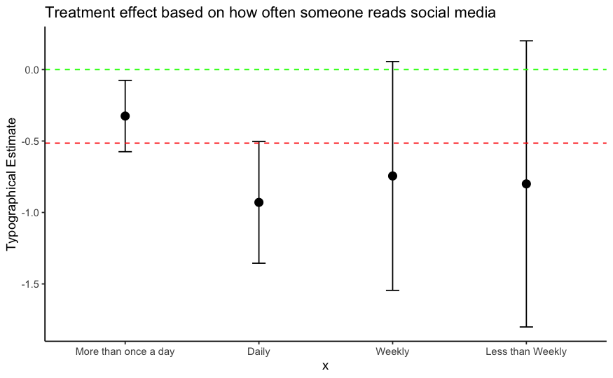
In order to understand whether individuals with different attributes have differences in their treatment effects, we decided to look at the estimated treatment effects and the confidence intervals associated with the estimates for individuals who read different levels of social media. We found that those who read social media posts at mid-frequency levels (weekly) tend to be more critical of phonological errors than those who read social media posts more frequently or less frequency. Those that read social media "More than once a day", "Daily", or "Less than Weekly", all have statistically signficant treatment effects with 95% CIs overlapping the average phonological treatment effect, but those that only read social media "Weekly" overlaps with 0. This could just be a coincindence though and should not be fully trusted without further studies.
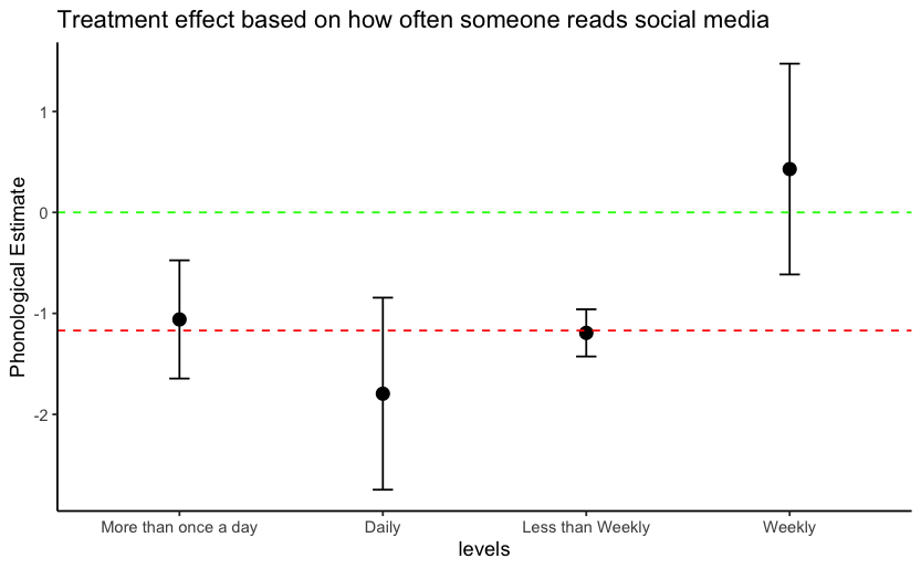
The same observation is not true for typographical treatment. While those that read social media posts "More than once a day" tend to have the weakest treatment effect, those who read posts more frequently tend to larger effects, although these estimates have large error bars.
Secondary outcomes -- Writing and effectiveness
As secondary outcomes, we wanted to see whether the perceived writing abilities of the authors and effectiveness of the posts were altered based on the treatment type. Interestingly, Writing abilities follows the exact same trend as Intelligence, where phonological treatment had nearly double the effect as typographical with both being statistically significant. However, effectiveness of the post was only different for the phonological group. This makes sense in a way: since intended words for typographical errors are usually easy to decipher, these typo do not obscure meaning. The effectiveness of posts with blatant phonological errors was severely impacted, although to a lesser extent than the impact for writing and intelligence. We leave these preliminary outcomes for potential future study.
| Dependent variable: | ||
| Writing | Effective | |
| (1) | (2) | |
| TreatmentPhonological | -1.334*** | -0.655*** |
| (0.106) | (0.104) | |
| TreatmentTypographical | -0.687*** | -0.062 |
| (0.115) | (0.115) | |
| Observations | 1,044 | 1,044 |
| R2 | 0.343 | 0.310 |
| Adjusted R2 | 0.319 | 0.285 |
| Residual Std. Error (df = 1007) | 1.277 | 1.399 |
| F Statistic (df = 36; 1007) | 14.580*** | 12.560*** |
| Note: | *p<0.1; **p<0.05; ***p<0.01 | |
Appendix: Bayesian Analysis
In addition to the frequentist analysis, we also conducted a brief exploration into Bayesian methods to better understand our data, modeling choices, and impact. In this section, we present two models: (1) a Bayesian estimation of our fully specified linear model, and (2) an alternative specification: an ordered logistic regression. Our analysis is powered by pymc3 and its requirements to replicate our results can be found in the repository's requirements.txt file. We leave this section mostly as future research and practice as the methods interest us while more work is still to be done.
Bayesian Linear Modeling
Estimating a Bayesian linear model shares some similarities with its frequentist counterpart, but differs in a few areas and comes with many advantages largely drawn from its estimation of a posterior distribution. The posterior distribution summarizes the relative plausibility of each possible value of the parameter and these values describe the relative compatibility of different states of the world with the data, according to the model. Further, it is useful to inspect the posterior distribution and to use it to generate samples of data so that we may better understand aspect of the data that are not well described by the model. As all models are wrong, we can use the posterior distribution to assess just how well the model describes the data.
In the code below, we: (1) load our data, (2) extract our observed outcome (y), (3) create two matrices for our treatment and covariates, and (4) we convert them to one-hot encoded vectors as they are categorical data.
# fully specified model
treatment_ucb = pd.read_csv('C:\\Users\\Andrew\\Desktop\\treatment_ucb.csv')

# extract y
obs_y = treatment_ucb['Intelligence']

# select useful vars
treatment = treatment_ucb['Treatment']
covariates = treatment_ucb[['Length', 'Gender', 'English', 'Race', 'isUS',
                            'Degree', 'age_bins', 'ReadSocialMedia',
                            'WriteSocialMedia', 'Intelligence.pretreat',
                            'Writing.pretreat', 'Interest.pretreat',
                            'Effective.pretreat']]

# onehot
treatment = pd.get_dummies(data=treatment, drop_first=True)
covariates = pd.get_dummies(data=covariates,
                               columns=[col for col in covariates.columns],
                               drop_first=True)
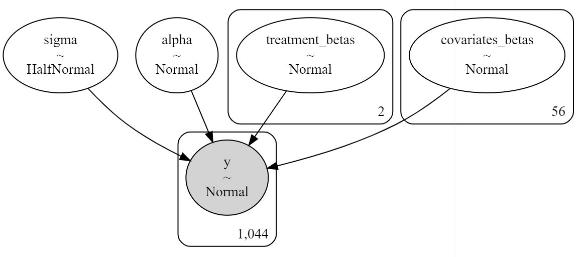
Next, we establish our model which contains several differences from frequentist statistics. First, we establish parameters by specifying their likelihood function, their expected value, the mu and sigma in the case of the Gaussian process, and their shape which is a way to conveniently create many variables at once. Setting good priors improves our black-box Markov Chain Monte Carlo sampler search process while also letting us envision how our prior estimates of the way the world works on our model, given the data.
# specify model
with pm.Model(coords=coords) as main_lm_model:
    '''
    linear model replication
    '''
    # priors
    alpha = pm.Normal('alpha', mu=0, sigma=1)
    treatment_betas = pm.Normal("treatment_betas", mu=0, sigma=1, shape=treatment.shape[1])
    covariates_betas = pm.Normal("covariates_betas", mu=0, sigma=1, shape=covariates.shape[1])

    # model error
    sigma = pm.HalfNormal("sigma", sigma=1)

    # matrix-dot products
    m1 = pm.math.matrix_dot(treatment, treatment_betas)
    m2 = pm.math.matrix_dot(covariates, covariates_betas)

    # expected value of y
    mu = alpha + m1 + m2

    # Likelihood: Normal
    y = pm.Normal("y", mu=mu, sigma=sigma, observed=obs_y, dims='obs_id')

    # set step and sampler
    step = pm.NUTS([alpha, treatment_betas, covariates_betas, sigma], target_accept=0.9)
Given our priors, we can draw samples and estimate its power to express our observed y.
# prior analysis
with main_lm_model:
prior_pc = pm.sample_prior_predictive(500)
# predictive prior plot function
def plot_prior(prior, model, group='prior', num_pp_samples=55):
ax = az.plot_ppc(
az.from_pymc3(prior=prior,
model=model
),
group=group, num_pp_samples=num_pp_samples,
figsize=(8, 8)
)
ax.set_xlim(1, 7)
ax.set_xlabel("Responses")
ax.set_ylabel("Probability")
return ax
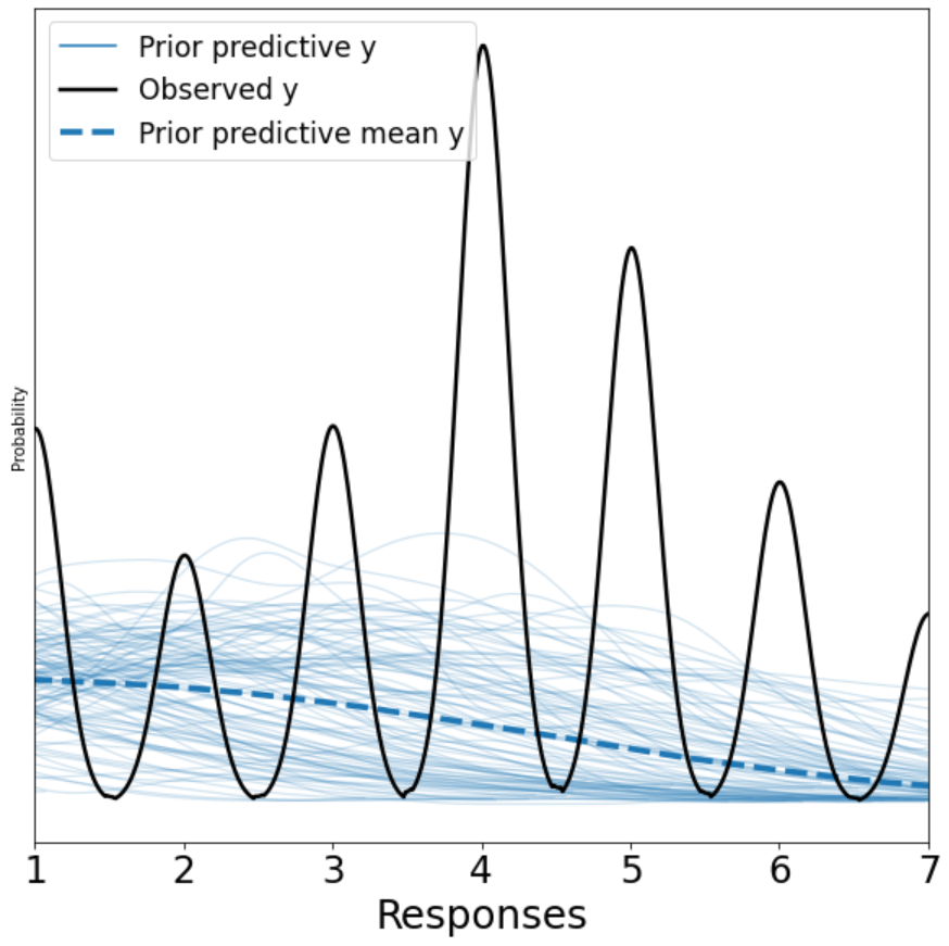
# doesnt fit well
ax = plot_prior(prior=prior_pc, model=main_lm_model, group='prior', num_pp_samples=100)
Ideally, we would want our observed outcome (the black line) to map nicely with our light blue traces representing the prior predictive y. We can see that this plot is likely telling us that a linear model is not the right model.
pymc3 also offers a nice convience function to display our precise modeling choices graphically, which we present below:
It is now time to (famously) hit our inference button and unleash the power of MCMC. In the code below, we: (1) draw 16000 samples (4000 samples per CPU core) to estimate the posterior distribution of our function, (2) initially draw 4000 samples (1000 samples per CPU core) in our search for parameters and delete them as part of the burn-in process.
# Inference button (TM)!
with main_lm_model:
    main_lm_model_idata = pm.sample(draws=4000,
                           step=step,
                           init='jitter+adapt_diag',
                           cores=4,
                           tune=1000,  # burn in
                           return_inferencedata=True)
# Sampling 4 chains for 1_000 tune and 4_000 draw iterations (4_000 + 16_000 draws total) took 161 seconds.
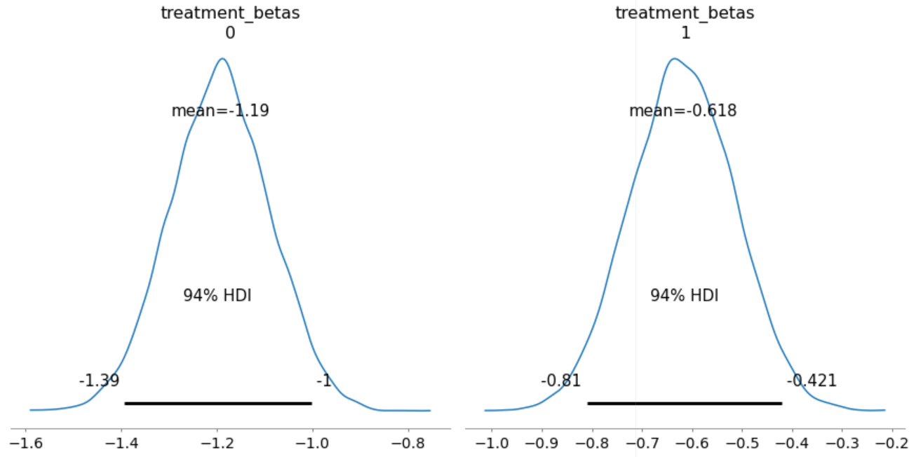
We are now ready to present our first quantity of interest for our treatment variables of interest Phonological and Typographical. The plot below is known as a High Density Interval which tells us that for density on the left (Phonological), 94% of the posterior probability lies between -1.39 and -1. This means that parameter values less than -1.39 or greater than -1 are highly incompatible with the data and model.
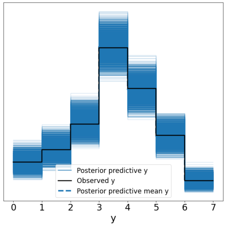
Next, we conduct one of the most powerful features of Bayesian data analysis: posterior predictive checks. In the code below, we generate 2000 data sets, each containing 1044 observations (the size of our data set); each drawn from the parameters estimated from our posterior distribution. The goal of this plot is to examine whether or not, after estimating our model's parameters, how well we can retrodict y.
# posterior predictive
with main_lm_model:
    ppc = pm.fast_sample_posterior_predictive(trace=main_lm_model_idata,
                                              samples=2000,
                                              random_seed=1,
                                              var_names=['treatment_betas',
                                                         'covariates_betas',
                                                         'y'])
Similar to our prior predictive plot, we find that we cannot generate data that looks like our outcome variable very well as the posterior predictions for y do match the patterns of our observed y.
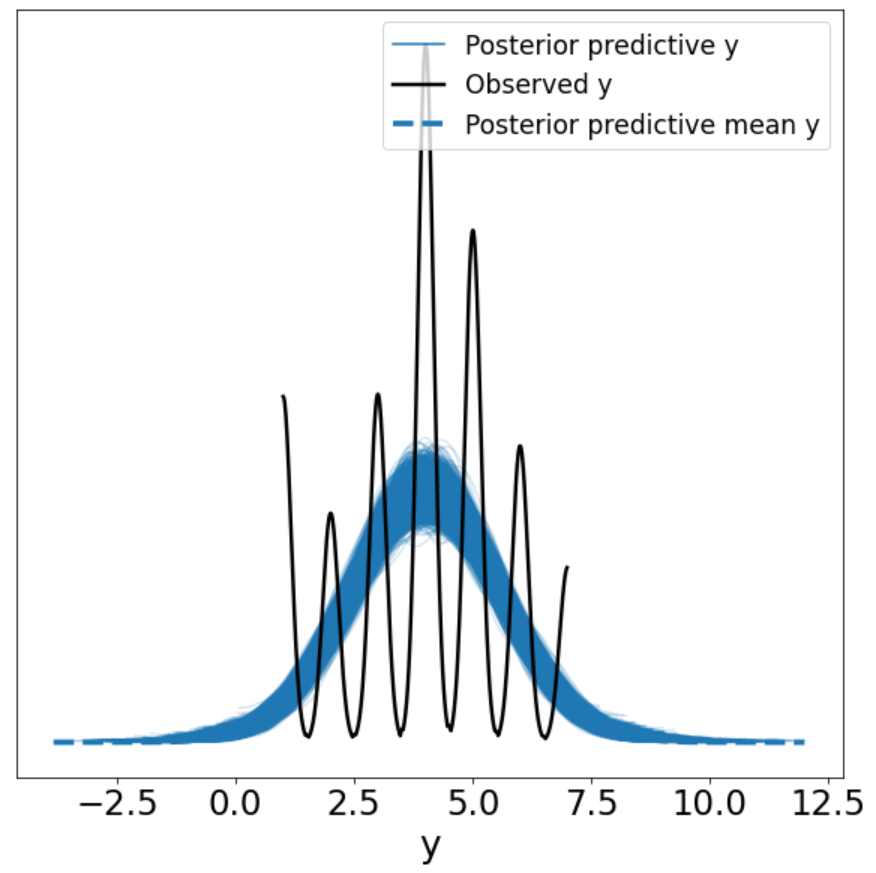
Bayesian Ordered Logistic Modeling
In modeling outcome values, we have to keep in mind that values are ordered, because 7 is greater than 6, which is the data that we have. Treating ordered categories as continuous measures is not a good idea as it might be much harder to move someone's preference from 1 to 2 than it is to move it from 5 to 6. The solution to this problem is to incorporate a cumulative link function that maps the cumulative probability of a value to that value or any value smaller. Put differently, the cumulative probability of 4 is the sum of the probabilities of 3, 2, and 1. In the steps below, we follow in a similar, albeit more complicated fashion as above.
The main difference here is that we are incorporating cutpoints which in effect act as our intercepts. Again we decide on prior values for their mu and sigma as they are drawn from the Normal distribution. By experimenting with different priors that fit the data, we can better help our sampler efficiently search in its effort to build a posterior distribution.
# specify model
with pm.Model() as cumlink:
    # priors
    cutpoints = pm.Normal("cutpoints", mu=[-5, -3, -2, -1, 1, 2], sigma=1, transform=pm.distributions.transforms.ordered, shape=6)
    treatment_betas = pm.Normal("treatment_betas", mu=0, sigma=1, shape=treatment.shape[1])
    covariates_betas = pm.Normal("covariates_betas", mu=0, sigma=1, shape=covariates.shape[1])

    # matrix-dot products
    m1 = pm.math.matrix_dot(treatment, treatment_betas)
    m2 = pm.math.matrix_dot(covariates, covariates_betas)

    # if we know m1 and m2, then we know phi
    phi = pm.Deterministic("phi", m1 + m2)

    # theano.tensor.sort(cutpoints) needed for prior predictive checks
    # Likelihood: OrderedLogistic
    y = pm.OrderedLogistic("y", eta=phi,
                           cutpoints=theano.tensor.sort(cutpoints),
                           observed=obs_y.values-1)

    # set step
    step = pm.NUTS([treatment_betas, covariates_betas, cutpoints], target_accept=0.9)
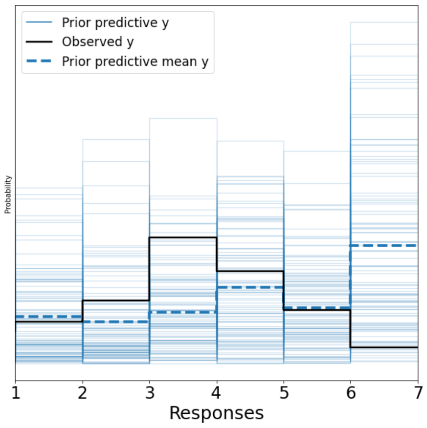
Our prior analysis reveals shows an improved fit and suggests that an ordered logistic regression is more likely to fit our observed data y as compared to a linear model.
# prior analysis
with cumlink:
    prior_pc = pm.sample_prior_predictive(500)

# priors look decent
ax = plot_prior(prior=prior_pc, model=cumlink, group='prior', num_pp_samples=100)
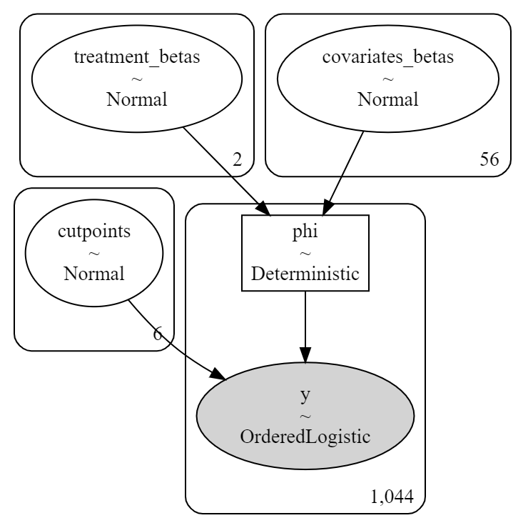
Similar to the linear model demonstration, we graphically summarize our modeling choices here:
Next we proceed to use our inference button:
# Inference button (TM)!
with cumlink:
    cumlink_idata = pm.sample(draws=4000,
                           step=step,
                           init='jitter+adapt_diag',
                           cores=4,
                           tune=1000,  # burn in
                           return_inferencedata=True)
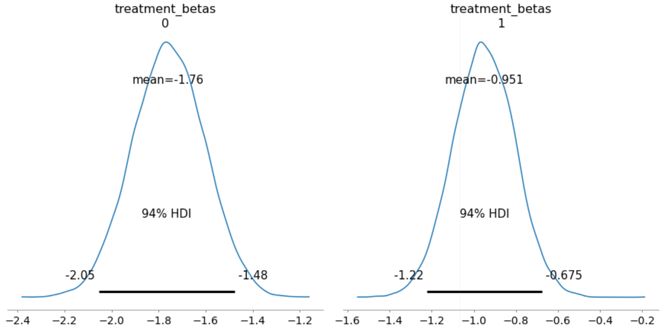
Our MCMC search finds that, as compared to the linear model, our primary variables of interest have a more pronounced impact. The image below shows that our coefficients move further away from zero while their mass contains slightly more plausible values. The HDI plot below tells us that, for the density on the right, (Typographical), 94% of the posterior probability lies between -1.22 and -0.675. This means that parameter values less than -1.22 or greater than -0.675 are highly incompatible with the data and model.
As you guessed, our next step is to determine how well our estimated parameters can recreate our observed data y. As a reminder, we are generating thousands of data sets and then visualizing it to see how well we can retrodict y.
# posterior predictive
with cumlink:
    ppc = pm.fast_sample_posterior_predictive(trace=cumlink_idata,
                                              samples=2000,
                                              random_seed=1,
                                              var_names=['treatment_betas',
                                                         'covariates_betas',
                                                         'y'])

# visualize model fit
az.plot_ppc(az.from_pymc3(posterior_predictive=ppc, model=cumlink),
            figsize=(8, 8));
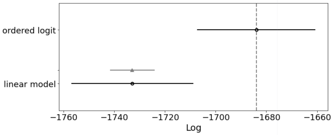
Next, we compare our two models according to Widely Applicable Information Criterion (WAIC) criterion. WAIC approximates the out-of-sample error that converges to the cross-validation approximation in a large sample. The value of the highest WAIC, (best estimated model), is also indicated with a vertical dashed grey line. For all models except the top-ranked model, the triangle indicates the value of the difference of WAIC between that model and the top model and a grey error bar indicating the standard error of the differences between that model and the top-ranked model.
# model comparsion
df_comparative_waic = az.compare(dataset_dict={"ordered logit": cumlink_idata, "linear model": main_lm_model_idata}, ic='waic')

# visual comparison
az.plot_compare(df_comparative_waic, insample_dev=False, figsize=(10, 4));
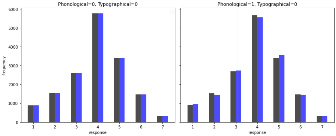
We now include a histogram of implied outcomes that we generate through simulating data from the posterior. Each plot shows how our outcome distribution varies by the primary independent variables. The black lines capture Phonological while the blue lines capture Typographical. The histogram shows the saliency of ordered categories. We can see that our control group is balanced while responses are weighted heavily on the middle response meaning meaning that a linear model most likely fail to adequately capture these differences.
Finally, in order to see whether an Ordinal Response model makes a difference in practice, we used the "polr" function from the MASS library to generate this model using a basic outcome against treatment model with no controls, and a model with the full set of controls (same as final specification described above). Here, we show the treatment and some of the pretreatment variables. Our conclusions do not change, and we get very similar coefficients with this model, indicating that in practice, the choice of modeling in this case does not make a difference on our conclusions.
| Dependent variable: | ||
| Intelligence (Ordered Factor) | ||
| No controls | With controls | |
| (1) | (2) | |
| TreatmentPhonological | -1.383*** | -1.764*** |
| (0.141) | (0.154) | |
| TreatmentTypographical | -0.675*** | -0.786*** |
| (0.134) | (0.147) | |
| Intelligence.pretreat | 0.324*** | |
| (0.060) | ||
| Interest.pretreat | 0.116*** | |
| (0.050) | ||
| Writing.pretreat | 0.254*** | |
| (0.079) | ||
| Effective.pretreat | 0.140*** | |
| (0.043) | ||
| Observations | 1,044 | 1,044 |
| Note: | *p<0.1; **p<0.05; ***p<0.01 | |
Potential Noncompliance
Treatment was successfully delivered to all individuals, but it is possible that treatment was not always properly received. On the flip side, Control subjects were all delivered posts with no typos, but the presence of typos may have been recognized anyway. As a result, we can make an argument that we have potential Defiers and Never Takers.
We define a subject as a compliers when they have both of the following characteristics:
- Recognized posts to contains errors when they were supposed to (Typographical or Phonological groups), and recognized posts as free of errors when none were present (Control).
- Must have actually read the post carefully. The average reader reads approximately 300 words per minute. We require the wmp to be between 50 (focused, one-session reading) and 500, which we feel are reasonable cutoffs. This in practice made much less of a difference than item 1, as most individuals fell between this region (see EDA).
Given these cutoffs, the complier rates in each group was: 78% Phonological, 76% Typographical, 63% Control.
For analysis of two-sided noncompliance, we used the 2-stage least squares approach with covariates described in here. We perform regression analysis with the same final model specification as above. CACE estimates and the standard errors are presented below for each of the treatment groups against with the control group as the base level. Generally, the CACE is higher than the estimated ATE from previous models assuming full compliance, with also larger standard errors. However, the conclusion as usual remains the same. Overall, no matter how we do the model interpret compliance, both treatment types are highly statistically sigificant, with the effect of phonological being about double the effect of typographical (although the ratio is slightly less here).
| Dependent variable: | ||
| Intelligence | ||
| Typographical | Phonological | |
| (1) | (2) | |
| CACE_estimate | -1.526*** | -2.734*** |
| (0.262) | (0.254) | |
| Intelligence.pretreat | 0.296*** | 0.172*** |
| (0.061) | (0.061) | |
| Observations | 719 | 689 |
| R2 | 0.313 | 0.377 |
| Adjusted R2 | 0.277 | 0.349 |
| Residual Std. Error | 1.203 (df = 683) | 1.219 (df = 658) |
| F Statistic | 8.871*** (df = 35; 683) | 13.282*** (df = 30; 658) |
| Note: | *p<0.1; **p<0.05; ***p<0.01 | |
Footnotes
-
Typographical errors, often known as typos, are spelling mistakes that occur due to slip of the hand when typing, and includes artifacts such as swapping letters, typing a letter close to the intended letter on the keyboard, or leaving out a letter. Usually the mispelled word is still easy to recognize. Examples include "somethimg", "hwo", and "thrd". Phonological errors on the other hand arise out of ignorance, or spellings based on sounds of the word. These usually demonstrate that the author truly does not know the proper spelling of the word. For example, "sumthing", "Kansus", and "razing". ↩
-
Please visit our public GitHub repository for the full data and analysis: Effect of Typographical and Phonological Errors in Social Media Posts on the Perception of the Authors' Intelligence ↩